We end this tutorial by introducing three additional functions that allow you to design a queueing system to achieve a specified level of service at the lowest possible cost.
Suppose that the owner of QTP Gas Emporium would like to ensure that 90% of the customers that enter the system wait less than 30 seconds before gaining access to a pump.
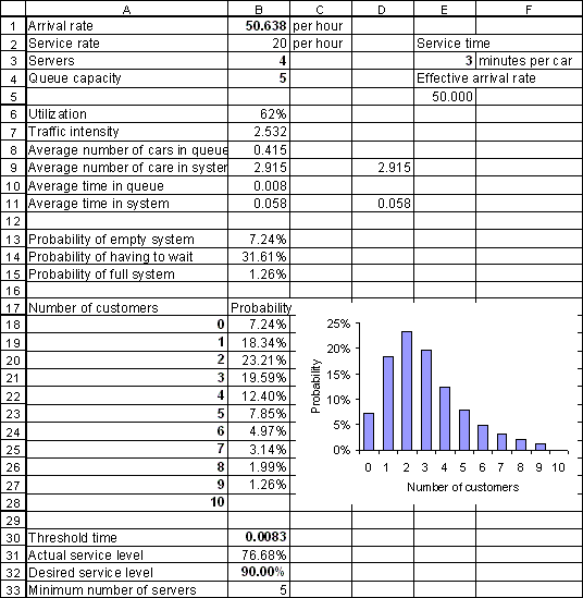
First, let us evaluate the current situation. The 30-second threshold time must be converted to hours (since the arrival and service rates are per hour). Thirty seconds equals (30 sec.)(1 min./60 sec.)(1 hour/60 min.) = 30/3600 hours. Enter "=30/3600" in cell B30 and "=QTPMMS_ServiceLevel(B30, B1, B2, B3, B4)" in cell B31. You will see that in the current system, 76.68% of customers who enter the system wait 30 seconds or less, while 100% - 76.68% = 23.32% wait longer.
Suppose that it is possible to add more pumps, but that each additional pump consumes one of the spaces in the queue. That is, the system capacity (number of servers + queue capacity) is fixed at 9. Under these assumptions, the QTPMMS_MinAgents function will tell you the smallest number of pumps needed to achieve the desired level of service.
Enter "0.90" in cell B32 and enter "=QTPMMS_MinAgents(B30, B32, B1, B2, 9)" in cell B33. The QTPMMS_MinAgents function should return 5. You can enter 5 in cell B3 and 4 in cell B4 to verify that if the number of pumps is increased by one and the queue capacity decreased by one, the service level rises from 76.68% to 91.80%, meeting the 90% objective.
The QTPMMS_MinServers function is similar to the QTPMMS_MinAgents function, except that it assumes that the number of servers can be changed without affecting the queue capacity. An airline check-in counter is an example of a situation where this assumption is appropriate.
Your spreadsheet should now look like this (columns H and I have not been included):

If you have successfully followed all the steps this far, you are well on your way to learning how to analyze waiting lines. Well done!