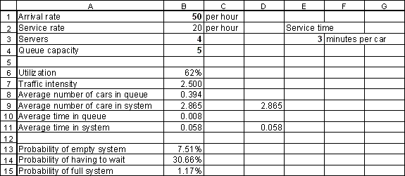
Now that we have entered the basic parameters that describe the queueing system we can begin to analyze its performance.
Enter the formula "=QTPMMS_Util(B1, B2, B3, B4)" in cell B6 and press Enter. Then select cell B6 and click the "%" icon on the formatting toolbar. Your spreadsheet should now look as follows:

The QTPMMS_Util function calculates the server utilization. A server utilization of 62% means that on average, each pump can be expected to be occupied 62% of the time and idle (or in other words, available) 100% - 62% = 38% of the time.
The cell references B1, B2, B3, and B4 are the arguments to theQTPMMS_Util function. They are, in order, the arrival rate, the service rate, the number of servers, and the queue capacity.
Different functions in the Queueing ToolPak have different arguments. The function wizard provides an easy way to see what functions are available in the Queueing ToolPak and what their arguments are. To do so, select the cell where you want the formula entered and then click the function wizard icon on the standard toolbar (the "fx" icon). Choose "Queueing ToolPak" in the function categorylist. This will display all the functions in the Queueing ToolPak. Selecting one of those functions will show what arguments it takes (for example if QTPMMS_Util is selected, thenQTPMMS_Util(Arrival_Rate, Service_Rate, Servers, Queue_Capacity)will be displayed).
Time-saving hint: Suppose you remember the name of a function but not its arguments. Select a cell, enter an equals sign and the name of the function, and then click the "fx" icon. This will open a dialog box showing the arguments to the function -- assuming you typed its name correctly!
Edit the formula in cell B6 to read "=QTPMMS_Util(-1, B2, B3, B4)" and press Enter. Cell B6 should now display the diagnostic error message that "#arrival rate < 0," i.e., the arrival rate argument is less than zero. Experiment with entering other invalid arguments, for example replacing B3 with 4.5. After you have finished experimenting, retype the correct formula "=QTPMMS_Util(B1, B2, B3, B4)" .
Next, enter the following four formulas in the cells indicated (click on the function names below for more information on each function):
Cell Formula
B7 =QTPMMS_TrafficIntensity(B1, B2, B3, B4)
B8 =QTPMMS_Lq(B1, B2, B3, B4)
B9 =QTPMMS_L(B1, B2, B3, B4)
B10 =QTPMMS_Wq(B1, B2, B3, B4)
B11 =QTPMMS_W(B1, B2, B3, B4)
Your spreadsheet should now look as follows:

These five calculations can be used to illustrate some fundamental relationships:
In cell D9, enter the formula "=B3*B6+B8" or in words, the "the number of servers times the average server utilization plus the average number of cars in queue." This quantity should exactly equal the average number of cars in the system (cell B9).
In cell D11, enter the formula "=B10+E3/60" or in words, the "average time in queue plus average service time (measured in hours)." As you might expect, this quantity should exactly equal the average time in system (cell B11).
Here are three more formulas to enter.
Cell Formula
B13 =QTPMMS_PrEmpty(B1, B2, B3, B4)
B14 =QTPMMS_PrWait(B1, B2, B3, B4)
B15 =QTPMMS_PrFull(B1, B2, B3, B4)
After entering the formulas, select the range B13:B15 and format it as percentages with two decimal places. Your spreadsheet should then look as follows:

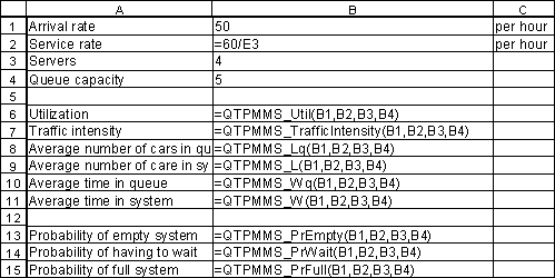
Press "ctrl" and "~" together to switch to formula view, which is useful for checking your work:

What do the probabilities you calculated mean?
There is a 7.51% probability that an observer that arrives at a random instant finds the system empty of customers.
There is a 30.66% probability that such an observer finds the system in a state where an arriving customer would have to wait, i.e., all the pumps are occupied.
There is a 1.17% probability that an arriving potential customer finds the system with 5 customers already waiting. As a result, the arriving potential customer will not enter the system to become an actual customer, i.e., he will balk.
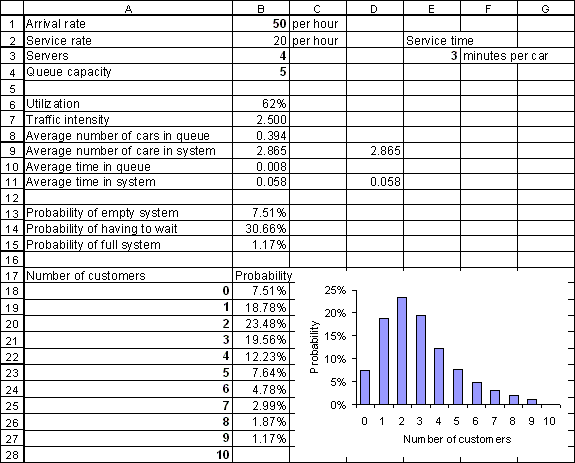
The QTPMMS_PrState function may help you gain a better understanding of the above three probabilities. The state of a queueing system (at least for so-called Markovian queueing systems) is the number of customers in the system. There can be at most 9 customers in the system we are analyzing (4 cars at the pumps and 5 cars waiting). Enter the numbers 0, 1, 2, ..., 10 in the range A18:A28. Then enter the formula "=QTPMMS_PrState(A18, $B$1, $B$2, $B$3, $B$4)" in cell B17 and copy this formula to the range B19:B28. This will calculate the probability that an observer arriving at a random instant sees 0, 1, 2, ..., 10 customers in the system. Format the probabilities as percentages and use the chart wizard to plot them, for example using a column chart. Your spreadsheet should then look something like this:

Note that cell B27 is blank. This is because the QTPMMS_PrState function returns nothing for states that are higher than the maximum number of customers in the system.
You can now check the following facts by making side calculations in the spreadsheet:
The state probabilities add up to exactly 100%.
The probability of the system being in state 0 is the same as the probability of the system being empty (cell B13 equals cell B18).
The sum of the probabilities of the system being in state 4 or higher equals the probability that a customer has to wait (cell B14 equals the sum of cells B22 to B27).
The probability of the system being in state 9 equals the probability that a potential customer will balk (cell B15 equals cell B27).
Note: The QTPMMS_PrWait function calculates the probability that an arriving customer enter the system and then waits for service. The probability that an arriving customer has to wait for service, given that (s)he enters the system (does not balk) can be calculated as (QTPMMS_PrWait - QTPMMS_PrFull)/(1 - QTPMMS_PrFull).
Now, it is time to revisit an assumption we have tacitly made up to now, namely that the arrival rate of 50 cars per hour that we used is appropriate. In fact, it is not, because it represents the average number of cars per hour that actually enter the system, rather than balk. This is because the company records only include customers that were actually served -- they do not include customers that arrived intending to purchase gas, but decided to go elsewhere when they saw that 5 cars were already waiting.
We will call the rate at which customers enter the system the effective arrival rate. In contrast, we will use the term actual arrival rate to refer to the rate at which customers arrive to the system, intending to enter it. The actual arrival rate includes customers that decide not to enter the system because of the number of customers waiting (i.e., customers who balk). Therefore, the actual arrival rate will always be larger or equal to the effective arrival rate.
All of the Queueing ToolPak functions require the actual arrival rate as an argument, rather than the effective arrival rate. To obtain the actual arrival rate from the effective arrival rate requires a bit of "reverse engineering" which we now describe.
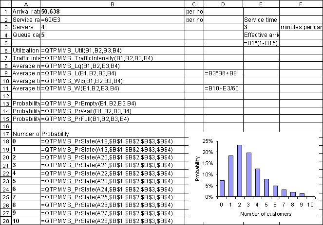
Imagine for a moment that the actual arrival rate is 50 cars per hour. Then we have already calculated that the probability of balking will be 1.17%. Therefore, the effective arrival rate will be 50*(1-0.017) = 49.42 cars per hour. Enter the formula "=B1*(1-B15)" in cell E5 to verify this. Now, you can experiment with the (unknown) actual arrival rate in cell B1 and observe what the resulting effective arrival rate will be in cell E5. Your goal is to make the effective arrival rate equal to 50. A bit of trial and error should convince you that the desired actual arrival rate is 50.638 cars per hour. (Note: it is possible to use Excel’s Goal Seek or Solver to do the work for you). Enter this value in cell B1. Observe that the performance measures you have calculated change slightly as a result of this. Your spreadsheet should now look like this, in formula view:
